🧬 Evolutionary Dynamics Simulator

What This Tool Does

This interactive simulator explores how complex patterns and behaviors can emerge from simple, local rules. At its core, it is a 2D evolutionary environment where each pixel represents a tiny agent — a "creature" or "cell" — which interacts with its neighbors according to a specified set of rules. These rules are defined in short, editable JavaScript files and determine how each agent evolves, competes, or dies based on the conditions around it.

The system illustrates a general principle: a rule-based, indeterministic autoencoder in which agents continuously transform and encode environmental information through interaction. Patterns appear, dissolve, self-organize, or collide — not by global orchestration, but by the accumulation of local changes.

You can choose from several prebuilt rule sets (e.g., grass–cow–wolf–tiger interactions), each capturing a different ecological or sociological metaphor. Or you can dive deeper, edit existing algorithms, or write your own to simulate any world you imagine.

The Logic of Evolution: How the Algorithm Really Works

This is perhaps the simplest kind of evolutionary simulation of its type — based on 1-to-1 local interactions. Yet even this minimal setup produces surprisingly rich dynamics.

Here’s how it works:

1. Initialization: A set of agents (each with a unique color and type ID: 0–6) is randomly scattered across the screen. This is triggered by clicking the Init button.
2. Evolution Loop Begins: When you hit Move or Run, the simulation enters a loop where each step represents one evolutionary action.
3. Agent Activation: A random pixel is selected. The agent at that pixel becomes "active" and gets to act. Other agents simply wait — no negotiation, no defense.
4. Local Interaction: The active agent randomly selects one of its 8 neighbors (its Moore neighborhood). Based on this neighbor’s type, it applies a predefined interaction rule. These rules are simple, deterministic, and editable by the user.
5. Rule-Based Outcome: Depending on the rule, the active agent might:
   • Transform the neighbor (e.g., “eat” or “kill” it)
   • Die due to isolation or starvation
   • Do nothing (based on probability or disallowed interaction)
6. State Update: The change is applied immediately — and the loop continues with a new random activation.

The key point: the agent isn't "smart." It doesn't think, plan, or sense more than one other entity. It simply reacts based on its interaction matrix. But even with such limitations, emergent dynamics appear.

And this is just the beginning. In this current version, only 1-on-1 local interactions are allowed. But future versions will include:

• Group dynamics
• History-sensitive behavior
• Delayed effects or memory
• Multi-step reasoning and reproduction strategies

You’re encouraged to explore and create your own rules — and see how far even simple logic can go.

How to Use the Tool

To begin, select one of the predefined evolutionary algorithms from the drop-down menu. Each algorithm defines a unique set of rules that govern how pixel-level agents interact with their neighbors — determining whether they reproduce, transform, die, or consume others based on their local environment.

Click the Init button to initialize the scene. Once initialized, use the Start, Move, and Stop buttons to control the simulation flow. You can adjust the speed of evolution using the Faster and Slower buttons.

Use your mouse wheel to zoom in or out — letting you observe the simulation at the individual pixel level or from a broader bird’s-eye view. You can also drag the scene to center on regions of interest.

To view the code behind any algorithm, click either the Open button on the right or the Algorithm button above. You can edit the algorithm directly within the interface — even while the simulation is running. This allows you to modify existing logic or experiment with entirely new behaviors in real time.

When you're satisfied with your custom version, use Save or Save As to store it. Your versions are saved in your browser’s local storage and persist indefinitely — no file system access is required. Everything is handled securely and locally by JavaScript.

The tool supports seamless switching between simulation, code, and statistical views. To see what's happening under the hood, click the Statistics button above the screen. Real-time metrics are updated every 100 milliseconds, including the proportion of agent types in the scene and the average number of neighbors of each type across all cells.

This tool is more than just a viewer — it’s a hands-on sandbox for exploring emergence, competition, adaptation, and chaos. Write your own rules. Watch your own world evolve.

Two Examples

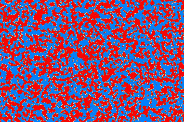
There are two algorithms in the list that I particularly like. One of them is algo_evo2, which stands out for its elegant simplicity. Despite its minimal setup, it helps answer a surprisingly compelling question: Who will win the battle between the reds and the blues? To answer it just let the algorithm run overnight — and by morning, the outcome will be clear to you. Below is a snapshot of what you might observe within just the first five minutes. You can enlarge images by right-clicking on them and opening in separate tabs. Note the sparkling yellow dots between the solid blue and red regions — they mark where the actual battles take place.

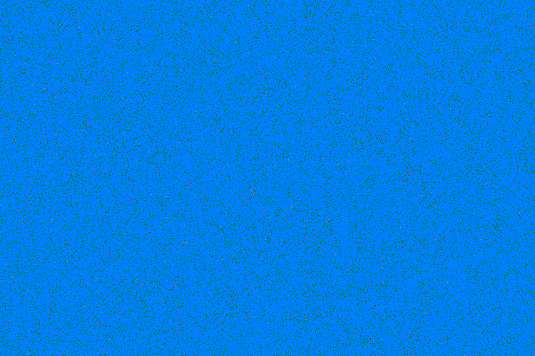
If you don’t really care about the outcome of that battle, then try another algorithm, which is also a favorite of mine: algo_evo4. I particularly like it for the interesting — and absolutely unexpected — collective behaviors it gives rise to. What emerges can only be described as distinct epochs or eras, each with its own character. Just when it seems like the system has stabilized, a new and entirely different behavior appears — unlike anything seen before. You can see how these epochs change in the images below: Top row: early phases (blue dominance, orange emergence, green takeover), and bottom row: transition to red clusters, structured red cores, total saturation system-wide blue phase → orange intrusions → collapse to green → emergence of red clusters → formation of red-core structures → complete red-core saturation.

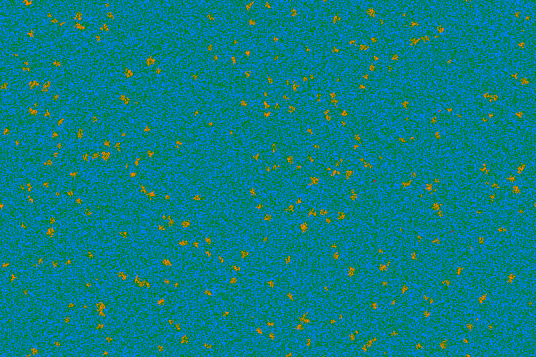
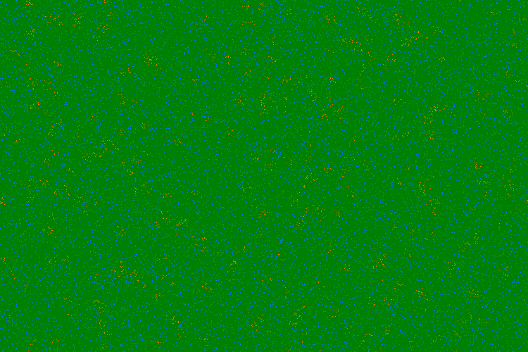
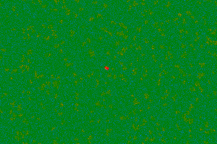
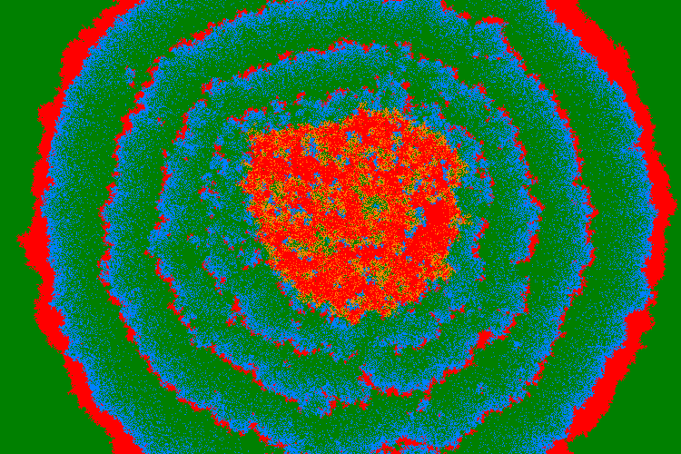
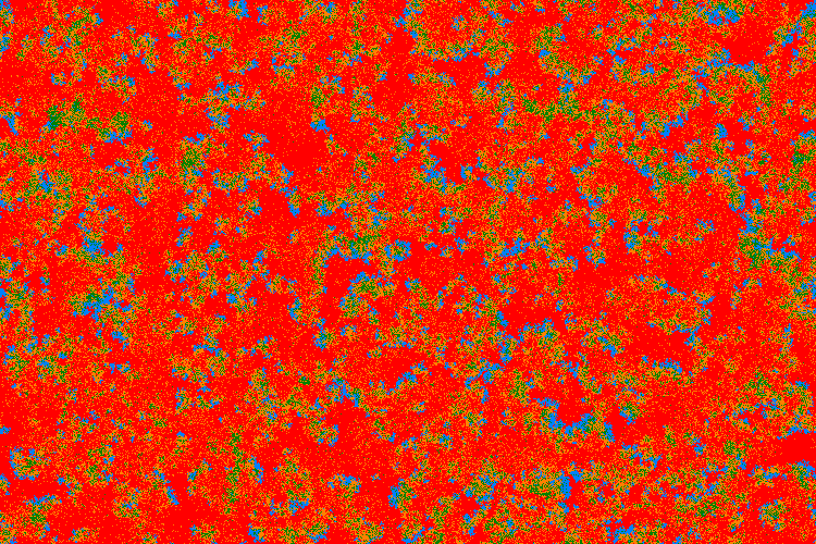
As you can see that the above six epochs are so different from one another, that it's hard to believe they all originate from the same simple and unchanging set of local rules.

Possible Interpretations

From a practical perspective, this first example can be seen as a highly simplified model of a territorial war. It represents an old-fashioned style of conflict — where battles are strictly local, and you can only eliminate your enemy through direct, face-to-face encounters. Modern wars, however, are mostly non-local, involving influence, reach, and action from a distance. This current algorithm doesn’t cover that kind of interaction — yet. But stay tuned — a demo of a non-local version is coming soon.

As to the second example, it can also be considered as an illustration to another pretty interesting real-world situations: the Emergent Dependency Chains with the Idea Spread or Supply Collapse.

Indeed, imagine a dynamic ecosystem where each layer of agents depends on the survival of the one below it. Four agent types are involved:

• 0: The passive substrate — empty space or ground-level potential
• 1: The base — early adopters, raw materials, or idea carriers
• 2: Mid-tier agents — processors, refiners, or idea developers
• 3: Top-tier agents — apex producers, influencers, or leaders

Each level spreads only by interacting with its specific feeder type: 3s grow only where 2s are present, 2s depend on 1s, and so on — forming a cascading chain of emergence. But with time, each layer also decays back to zero, leading to constantly shifting boundaries, bursts of organization, and collapse.

This behavior can model a range of real-world systems:

• 🔄 Social learning: From idea exposure to widespread adoption and eventual burnout
• 🏭 Economic systems: Layered production chains where failure at one level triggers upstream collapse
• 🧠 Learning systems: Knowledge building atop prior concepts — but fragile if foundations are lost

Try this demo under the algorithm name algo_evo4 and observe the striking frontiers, looping patterns, and complex rippling structures that emerge — all from just a few simple local rules. You can also modify it, and add your own rules, if you want. The tool allows one to do that.

Why JavaScript?

This simulator was originally developed decades ago as a DOS-based C program. Today, it's reimagined in JavaScript — a language perfectly suited for experimentation, real-time visualization, and web-native interaction. With JavaScript, you can update the rules, rerun the simulation, and instantly observe the result — no need to recompile or refresh.

Every algorithm is self-contained in a short `.js` file, making it easy to understand, modify, and share. By using pixel-level graphics and asynchronous interactions, the system strikes a balance between visual intuitiveness and algorithmic flexibility.

How the JavaScript Code Works

One of the strengths of this simulator is its modular design. The main evolution engine — which controls timing, visualization, and neighborhood scanning — is completely isolated from the logic that defines how agents behave.

The behavior rules (interaction logic) are defined in small JavaScript files — one per algorithm — and can be edited, extended, or created from scratch. This makes it easy for anyone to experiment by defining new dynamics, without needing to touch the main simulation code.

What a Rule File Looks Like

Here's an excerpt from one of the built-in algorithms, algo_evo4.js:

	function proportion()
	{
		return [100, 5, 1000, 1];
	}
	
	function algorithm(x) 
	{
		var a1 = 1.0, a2 = 1.0, a3 = 1.0;
		var m1 = 0.00, m2 = 0.05, m3 = 0.05;
	
		var y = x;
		if (x[0] == 1) {
			if (Math.random() >= a1) return y;
			if (x[1] == 0) y[1] = 1;
			if (Math.random() < m1) y[0] = 0;
		}
		else if (x[0] == 2) {
			if (Math.random() >= a2) return y;
			if (x[1] == 1) y[1] = 2;
			if (Math.random() < m2) y[0] = 0;
		}
		else if (x[0] == 3) {
			if (Math.random() >= a3) return y;
			if (x[1] == 2) y[1] = 3;
			if (Math.random() < m3) y[0] = 0;
		}
		return y;
	}
	

What This Code Means

• proportion() defines the initial mix of agent types. In this case: lots of 2s, a few 1s, and very few 3s.
• algorithm(x) defines how a pixel of a certain type (x[0]) acts on its neighbor (x[1]).
• Each agent type can:
  • Interact with a specific other type (e.g. 2 → 3 only if neighbor is 2)
  • Possibly change that neighbor into its own type
  • Randomly die (revert to type 0), based on a mortality rate

You can edit this code directly inside the simulator interface. Simply click the "Open" button next to an algorithm, make changes, and save a new version to run it immediately. This sandbox-style workflow makes it easy to explore hypothetical rules, tweak behaviors, or create new worlds from scratch.

What’s Coming in the Next Demos

This simulator is a conceptual playground — a way to experiment with how rules shape behavior and how emergence happens from the bottom up. What you see here is the simplest version of the algorithm: agents interact one-on-one with randomly selected neighbors, following predefined static rules.

More advanced versions will follow soon. They will explore:

• Extending from 1-to-1 to 1-to-8 Moore neighborhood interactions
• Replacing static rules with adaptive, learning-based behavior
• Incorporating resource-aware optimizations (like energy or memory constraints)
• Introducing individual traits and identities
• Modeling intelligence, memory, and strategy

While this current version is abstract and agent-based, these same models can apply to real systems — from biological organisms to economic agents, social networks, or ecological competition.

You’ll soon see new use cases based on:

• The spread of diseases or ideas
• Cooperation and competition in social systems
• Evolution of cultural or institutional behavior
• Multi-agent learning and emergent decision loops

🎬 Curious what happens when agents represent real biological systems — and entire neighborhoods interact by competing for limited resources? Here’s a visual story of cows, wolves, and tigers that shows a next-level algorithm in action:

👉 Read the Visual Essay: “Evolution on the Screen”

More demos, smarter agents, and deeper dynamics coming soon. Stay tuned.